

What Are Data and Data Visualization?
Data is information that we collect about the world. In the context of NOAA Ocean Exploration, it is the information that we collect about the deep sea. Data can be both quantitative and qualitative. Quantitative data refers to information that is numeric: it is anything that can be counted or measured. In the deep sea, quantitative data types can include things like the number of fish seen or the area covered by deep-sea corals. Qualitative data is more descriptive and refers to things that can be observed but not necessarily measured numerically. For example, in the deep sea, we may collect qualitative data about the behavior of a particular organism.
Data visualization is the representation of data through the use of graphics such as charts, plots, pictures, or graphs compared to text alone.
Images and graphics are effective for all kinds of storytelling, especially when the story is complicated, which is often the case in science. Data visualization can also allow us to see trends and patterns in the data that we might not see if we were just looking at numbers alone. Scientific visuals can be essential for analyzing data, communicating results, and for making new discoveries.
Examples of Different Data Visualizations


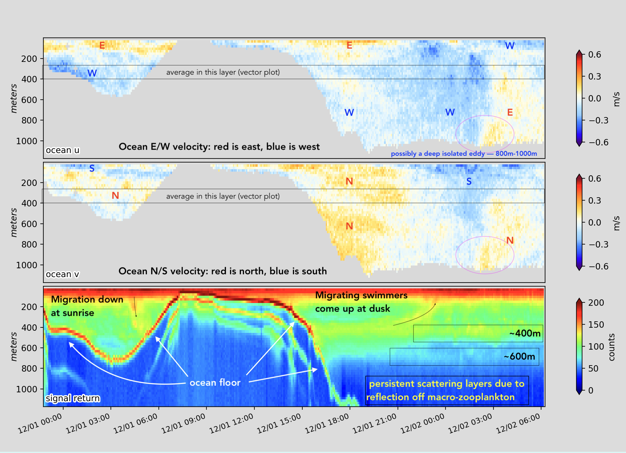
Example of Acoustic Doppler Current Profiler (ADCP) velocities with depth. This color panel plot shows three panels with horizontal velocities in the east-west (E/W) direction (top panel), north-south (N/S) direction (second panel) and signal return (bottom panel). Time increases from left to right as the ship transits to the northwest (same data as the vector plot, above). The vertical axis is depth in meters. Image courtesy of NOAA Ocean Exploration. Download largest version (jpg, 805 KB). Learn more
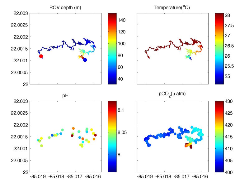
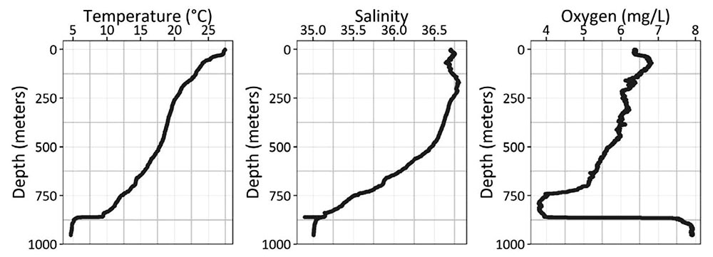
Remotely operated vehicle (ROV) track and the measured parameters from an ocean exploration dive: (top left) depth (meters), (top right) temperature (°C), (bottom left) pH, and (bottom right) dissolved carbon dioxide (pCO₂; in microatmospheres or µatm). Blue and red dots indicate the start and end of the dive. The ROV first dove to around 150 meters (492 feet) at the base of the reef (blue dot in the top left panel), slowly climbed the reef wall and then moved around on top of the reef. Spatially the ROV covered about 300 meters (984 feet) in the west-east direction and less than 100 meters (328 feet) north-south over a period of approximately 3 hours. Image courtesy of Undersea Vehicles Program, University of North Carolina Wilmington, Cuba’s Twilight Zone Reefs and Their Regional Connectivity. Download largest version (jpg, 343 KB). Learn more
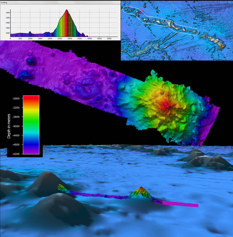
Composite image showing the original Sandwell and Smith satellite-derived bathymetry data at the bottom, with NOAA Ship Okeanos Explorer EM302 multibeam bathymetry transit data further revealing this unnamed seamount overlain on top. The middle image is a top-down view of the bathymetry data showing the seamount, and the graph in the upper left corner shows the vertical profile of the seamount’s height relative to the seafloor. The map on the upper right shows the bathymetry of the Hawaiian Archipelago with the Papahānaumokuākea Marine National Monument boundary in white, and the location of the seamount circled in red. Image courtesy of NOAA Ocean Exploration, 2015 Hohonu Moana. Download largest version (jpg, 1.4 MB). Learn more
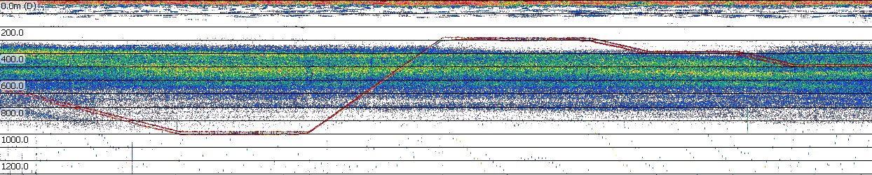
This is an example of what the deep-scattering layer looks like when graphed as an echogram, which is a plot of active acoustic data. Warmer colors indicate more backscatter, meaning that more (or stronger) echoes were received back from the organisms at that depth. The red line indicates the remotely operated vehicle trajectory as it performs transects throughout the layer. The scale on the left represents depth in meters. Image courtesy of NOAA Ocean Exploration. Download largest version (jpg, 584 KB). Learn more
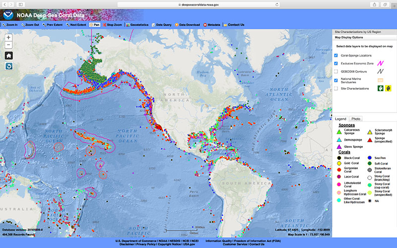
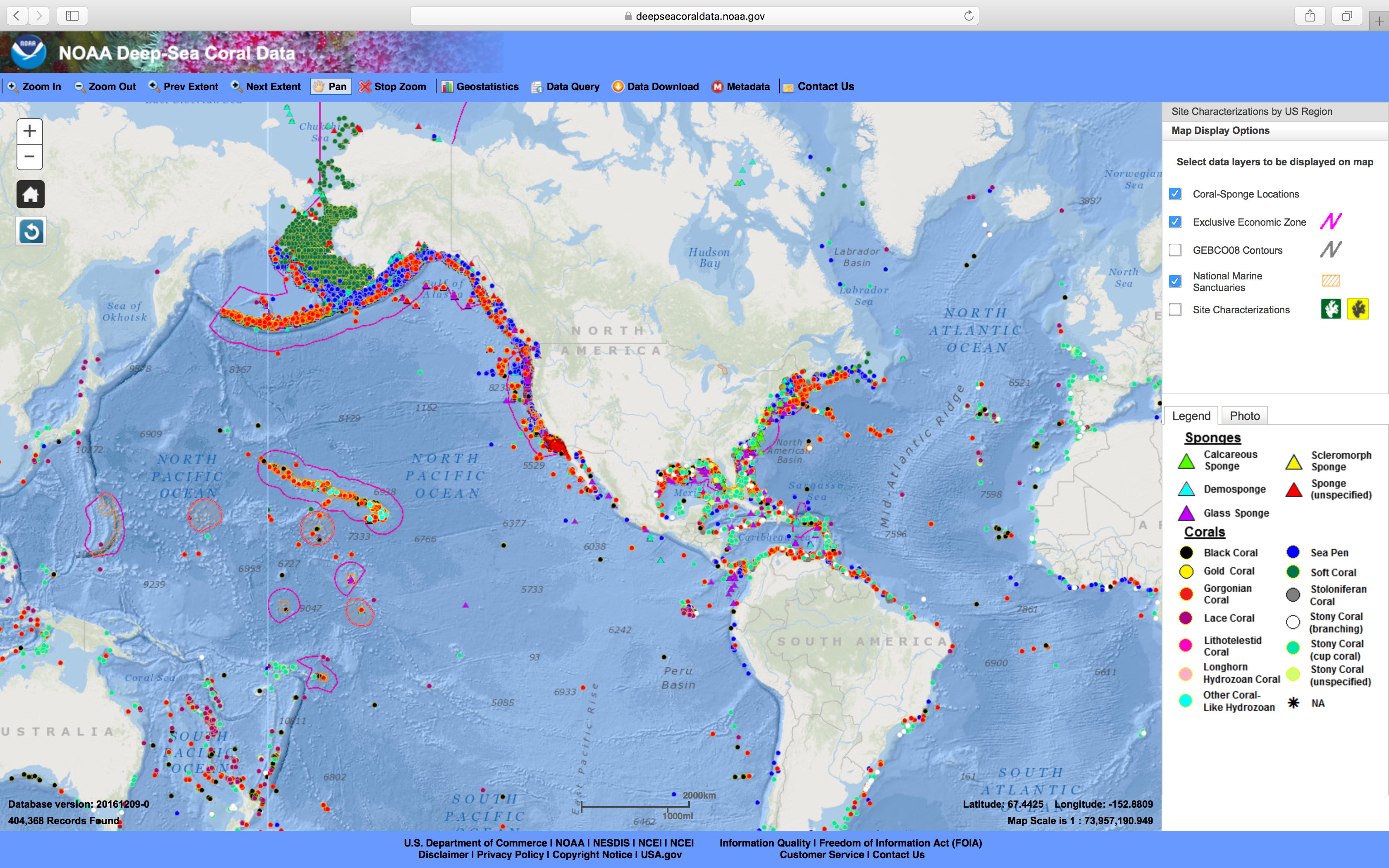
Deep Sea Coral Data Portal digital map showing known locations of corals (circles) and sponges (triangles). Coral and sponge location records are tagged with metadata and many have associated photographs available as well. Note that the map does not yet show areas in which researchers have searched and found no coral. Image courtesy of the NOAA Deep Sea Coral Research and Technology Program. Download largest version (jpg, 3.1 MB). Learn more
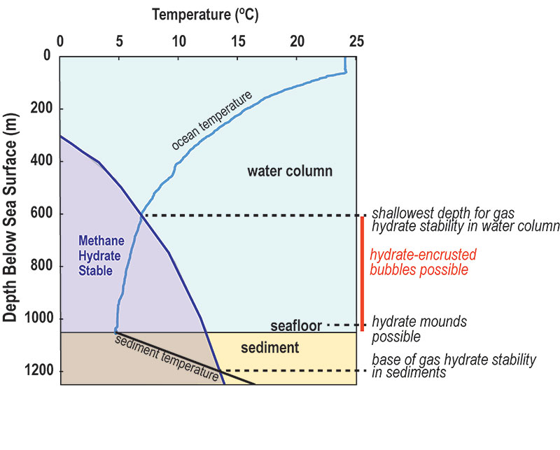
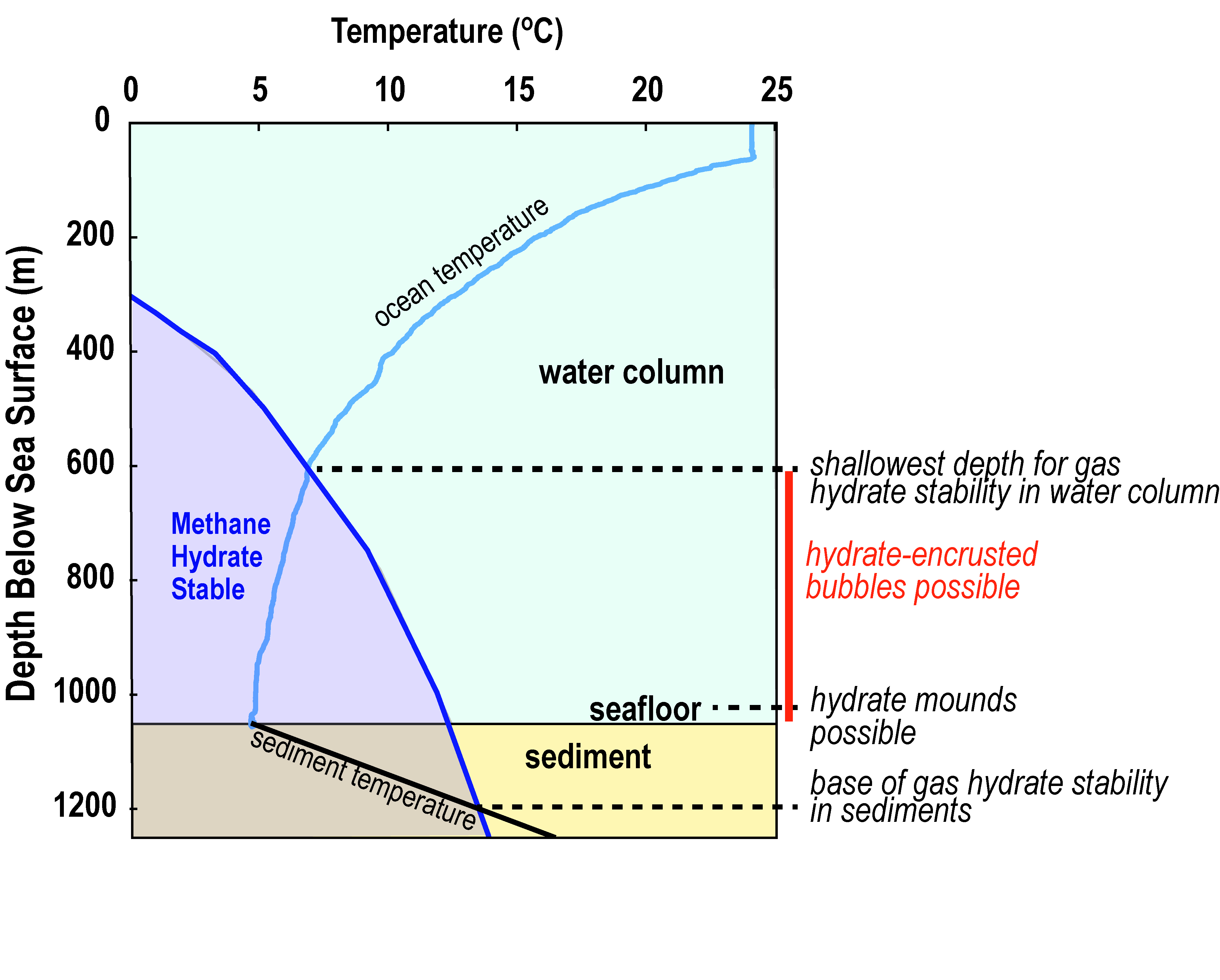
Methane hydrate is stable to the left of the purple curve on this temperature-depth plot. Each 100-meter (328-foot) increase in water depth corresponds to a pressure increase of approximately 10 megapascals (98 atmospheres). The blue curve shows the ocean temperatures measured by the conductivity-temperature-depth (CTD) sensor on remotely operated vehicle Deep Discoverer. The sediment temperatures are estimated based on a study that examined nearby well data. Gas hydrate is stable at the seafloor, in the shallow sediments, and from the seafloor to approximately 600 meters (1,967 feet) depth in the water column. Such conditions are typical for the deep ocean, but the Gulf of Mexico leaks such large volumes of gas that near-seafloor gas hydrate is more common there than in most locations. Diagram provided by C. Ruppel, U.S. Geological Survey. Download largest version (jpg, 1.9 MB). Learn more


