


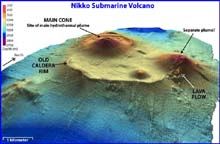
Nikko submarine volcano has two summit cones within the remnant of a large circular caldera, which has been subsequently filled by eruptive material. Click image for more information and larger view.
Seafloor Mapping
Bob Embley
Geophysicist
NOAA, Pacific Marine Environmental Laboratory
Producing maps of the seafloor has always been a particular challenge to humankind. The first primitive maps came from successions of single soundings produced by lowering weighted lines into the water and noting when the tension on the line slackened. By measuring the amount of line paid out, one could determine the depth. These early maps gave only the most general picture of the ocean floor, and only the larger features could be identified by looking for patterns in many such soundings. Most of these surveys were conducted to identify near- shore hazards to shipping. Only in the late nineteenth century did expeditions begin to take large numbers of soundings in deep water.
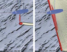
Comparing single (left) and multibeam (right) echo sounding of the seafloor. The multibeam method is preferred because it measures an entire area rather than a single line of seafloor. Click image for a larger view and a more detailed explanation.
The first modern breakthrough in seafloor mapping came with the use of underwater sound projectors called “sonar,” which was first used in World War I. By the 1920s, the Coast and Geodetic Survey (the predecessor agency to NOAA’s National Ocean Service) was using sonar to map in deep water. The team of A. C. Veatch and P. A. Smith produced one of the first detailed maps of the ocean floor. This map showed that the canyons off the East Coast of the United States extended into very deep water.
During World War II, advances in sonar and electronics led to much improved systems that provided precisely timed measurements of the seafloor in great water depths. These systems provided the databases used to construct the first real maps of important features, such as the deep-sea trenches and mid-ocean ridges. The 1957 publication of Heezen and Tharp’s physiographic map of the North Atlantic was the first map of the seafloor that allowed the general public to begin to visualize the ocean floor. These early maps based on hundreds of thousands of hand-picked depths provided the context for the plate tectonics revolution in the 1960s that finally gave scientists satisfying explanations for the formation of mid-ocean ridges, trenches, mountain ranges and the “ring of fire” around the Pacific.
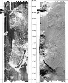
Heceta Bank Simrad EM 300 backscatter (left) and topography (right) on 10m grids. The backscatter image reveals seafloor physical properties and texture of the seabed. White areas depict cobble, boulder and sand areas. Black areas depict muddy areas. Click image for larger view and more detailed information.
Still, these systems only produced depth soundings immediately below the ship’s tracks. To produce maps of the shape of the seafloor, one had to laboriously “contour” an area by connecting lines of equal depth together. Although the advent of digital computers in the 1960s provided much needed automation for plotting data, the civilian scientific community was still using the same basic technology until the 1970s.
In the 1960s, the U. S. Navy began using a new technology of “multibeam sonar." Arrays of sonar projectors produced soundings not only along the track, but also for significant distances perpendicular to the ship’s track. Instead of lines of soundings, these new multibeam systems produced a swath of soundings. Combined with automated contouring, the ability to make detailed, complete maps of large areas of the seafloor became available to the scientific community for the first time in the late 1970s after the Navy declassified the technology. Since these first multibeam systems, this technology has steadily improved, and modern systems can map swaths up to several times the water depth. Combined with positional information gained by the geographic positioning navigation systems and advanced computer graphics, these systems now provide a whole new view of the seafloor.
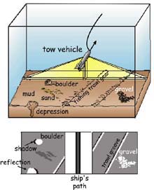
Schematic diagram of a sidescan sonar towed instrument scanning the seafloor (top) and the sidescan data record created (bottom). Click image for larger view and a more detailed explanation.
Knowing the shape of the seafloor is critical to advancing our knowledge of the ocean. It is also critical that we map changes in the composition of the seafloor. However, whereas the depth can be measured using the timing of the signals going to and from the seafloor, a precise measurement of the “strength” of the sonar return is needed to determine the texture of the seafloor. For example, a sound pulse impinging on a mud seafloor will be mostly absorbed with only a small percentage returning to the receiver. But a rock bottom will absorb very little sound and return most of it. In this way, modern seafloor survey systems measure relative strength of signal return as well as the depth. The record that results consists of a pattern of variable strength signal returns that illustrate the seafloor’s composition.
An alternative method of mapping the texture of the seafloor is provided by a “sidescan sonar” system. These systems are towed on cables, and send and receive sound signals over a broad swath of seafloor. The sonar arrays are positioned in such as way that they project sound at low angles. The resulting record can detect very subtle features by the acoustic “shadows” that are cast. Depending on the pitch of the system (low pitch sound travels farthest), sidescan sonar can cover hundreds of meters to kilometers of seafloor.
Using a sonar array mounted on the hull of a research vessel to map the seafloor has advantages. The vessel can travel at about 10 knots (~18.5 km/hr). It is very stable, and the data is generated in near real time and can be processed into useable maps very quickly. However, as the water depth increases, the “footprint” of the beams generated by the sonar become larger, similar to the spreading out of the beam of a flashlight with distance. Because the sonar averages the echo return across each beam to generate a depth point, the spreading out of the beams decreases the resolution of the resulting map. With increasing depth, there is an another limitation as well. The higher frequency sound needed to generate very accurate maps increasingly loses energy (“attenuates”) as it passes through more and more water.
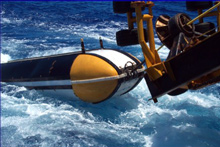
The MR1 towed long-range sidescan sonar system, which will be used to map the submarine volcanoes in the Marianas arc. Image courtesy of Hawaii Mapping Research Group. For more information about the MR1 system click here. ![]() Click image for larger view and a detailed explanation.
Click image for larger view and a detailed explanation.
During the Submarine Ring of Fire project in 2003, we will be using a towed long-range sidescan sonar system called MR1 to map the submarine volcanoes in the Marianas arc. The MR1 sonar will be towed behind the ship at a depth of about 100 meters, while the ship travels forward at 9 knots. The MR1 data will help us understand the recent history of each volcano by revealing lava flows, landslides, and faults. MR1 is operated by the Hawaii Mapping Research Group at the University of Hawaii. While we are surveying with MR1, we will also be collecting bathymetric data with the R/V Thompson's EM300 multibeam sonar system. This bathymetry will show the shape and depth of each surveyed submarine volcano. It will be very important for conducting our CTD/plume-mapping operations this year and will help us plan our remotely operated vehicle dives to some of these volcanoes next year.